Table of Contents
- Installation
- Simple practice
- Lessons from Tania
- R packages
- Load spreadsheet data (csv and Excel files)
- Dataframe manipulation including subsetting, merging
- Write data
- Functions introduction
- Free R courses and learning tools
Installation
- Install R, the free behind-the-scenes code that allows your computer to run R scripts
- Pick a local mirror site from The R Project for Statistical Computing website (any is fine)
- Select your operating system, "Download R for..."
- Install the "base" distribution of R
- This is the actual R programming language software
- Install RStudio, the user interface software
- Get free RStudio Desktop. Install this after you install R (not before).
- Ignore the paid versions, RStudio Desktop Pro and RStudio Server. You don't need those.
- Default settings are ok
- RStudio is an optional but very helpful tool
- Once you have both installed, you can open RStudio Desktop and it will automatically detect your version of R language.
Simple practice
- Open RStudio and try replicating the console commands below. Note that integer lists are written as beginning:ending separated by a colon (e.g. 1:10 means 1,2,3,4,5,6,7,8,9,10).
- To assign values to variables, R allows either an equal sign or an arrow:
- x <- 1:10
- x = 1:10
- These two things both assign an integer list of 1 to 10 to the variable x.
- Once you have assigned the values to x, you can now create a new variable y which uses the values of x.
- y <- x^2
- This creates variable y with a list of values 1,4,9,16,25,36,49,64,81,100.
- With two number variables of equal length like our example x and y above, you can create a scatter plot.
- plot(x,y)
- The plot function also allows some customization such as selecting the point colors.
- plot(x,y,col="red")
- Note that "red" must be in quotes because it is a value, not a variable. You are assigning the value "red" to the function's variable col. This would also work:
- mycolor = "blue"
- plot(x,y,col=mycolor)
- In this case you don't need the quotes since you are passing the value of variable mycolor to variable col. That value is "blue", which R understands as one its named colors.

- You can learn more about the plot function (or any function) by looking at the R help files.
- Type "?" and the function name into the console window and hit Enter. For example:
- ?plot
- This opens a Help tab with information about the function.

- Read the ?plot help window and try formatting the plot in different ways.
- col = color for points (can be named values like "red" or hex codes)
- pch = point type (asterisks are pch=8)
- Try different math functions.
- Comments in R begin with a hashtag (#). Nothing after the "#" is run as a script.
- Variable values can be set with an equal sign (=) or an arrow (<-) in R.

Lessons from Tania
R packages
R comes with a pre-loaded set of functions, practice datasets, and variables (e.g. pi = 3.141593). This set of tools is called base R.You can also download additional tools by installing packages. Using packages requires two steps:
- Install the package. This is like installing software on your computer, but you do it through RStudio. You only need to do it once, unless there's an update and you want to install the new version.
- Load the package. Do this every time you open a new R session and need the package. This is like opening already-installed software. If you close RStudio, go to lunch, and come back, you will need to load the package again. If you try to run a package-specific function, you will get an error message if you forgot to load the package.
- CRAN: The Comprehensive R Archive Network
- install.packages("ggplot2") #this installs "ggplot2", an advanced plotting package
- library("ggplot2") #this loads the package
- Bioconductor: open source software for bioinformatics
- if (!requireNamespace("BiocManager", quietly = TRUE))
- install.packages("BiocManager") #first step to install Bioconductor tools
- BiocManager::install("biomaRt") #second step to install the "biomaRt" package
- library("biomaRt") #this loads the package
x=1:10y=x^2qplot(x,y)
x=1:10y=x^2ggplot2::qplot(x,y)
Load spreadsheet data
Text-based spreadsheets import (recommended)
It is easier to load your spreadsheet data as a text file (.txt), comma-delimited file (.csv), or tab-delimited (.tsv) file. You only need base R and it loads faster than Excel files.Two methods to load text-based files (.txt, .csv, .tsv):
- Manually load using RStudio: File >> Import Dataset
- Load through the RStudio console using one of the lines of code below:
df = read.table("myfile.txt", stringsAsFactors=FALSE)
df = read.csv("myfile.csv", stringsAsFactors=FALSE)df = read.csv("myfile.tsv", stringsAsFactors=FALSE, sep="\t")df = read.csv(file="myfile.csv", header=TRUE, skip=2, stringsAsFactors=F)
Use sep to specify how values are separated (sep="\t" for tab-separated values). The default is comma-separated (sep=",") for read.csv so you don't need to include it if that's what you need also. You can view other defaults by typing ?read.csv into the RStudio console.
Excel spreadsheets import
Beware: loading Excel spreadsheets takes much longer than simpler text-based formats. For small spreadsheets, the difference is negligible (seconds). For large datasets with thousands of columns, you may have issues (1 minute csv file vs 30+ minutes for the Excel file).#install.packages("gdata") ##commented out so it won't run## to run the above line, remove the hashtag in front of itlibrary(gdata) ## load the gdata packagedf = gdata::read.xls("myspreadsheet.xlsx", header=TRUE,stringsAsFactors=FALSE, skip=0,sheet=1)
The sheet part is required so you can specify which sheet (number) you want to use since Excel spreadsheets can have different sheets. Most other settings are optional.
If you get a perl-related error, you may need to specify the path where perl is installed. Example:
perl = "C:/Strawberry/perl/bin/perl5.26.1.exe"
      df = read.xls("myspreadsheet.xlsx", header=TRUE,
                     stringsAsFactors=FALSE, skip=0, sheet=1,
                     na.strings="NA",
                     method="csv", perl=perl)
The na.strings part is telling the function what values are equal to not available (NA) values. Otherwise, they may be imported as a string "NA" (literally the letters "N" and "A" rather than the no value meaning you want).
The method part specifies the method to use for data import. See alternatives by inputting ?read.xls at the console to read the function help page.
If you get an error "duplicate 'row.names' not allowed", fix it by removing columns with commas or changing your import method.
Dataframe manipulation
Quick functions to learn more about your dataframe
head(df) #print the first 6 rows of your dataframe
tail(df) #print the last 6 rows of your dataframe
dim(df) #print the number of rows and columns
View(df)
summary(df)
#provides simple math values for columns, e.g. min, max, mean, standard deviation
table(df$columnName)
#counts number of rows that match each value in the column, good for groups, not gene names
table(df$columnName1, df$columnName2)
#counts the overlap of categories in these two columns
table(df$columnName1, df$columnName2, useNA="always")
#counts the overlap of categories in these two columns, including any NA values
- df$columnName = as.character(df$columnName) ##string values
- df$columnName = as.numeric(df$columnName) ##number values
- df$columnName = as.factor(df$columnName) ##factor values
- df$columnName = as.logical(df$columnName) ##TRUE/FALSE
Subsetting dataframes
- dfsub = subset(df, pvalue<0.05)
- dfsub = subset(df, biotype=="protein_coding")
- dfsub = subset(df, tissue=="CVS" | tissue=="Placenta") #example 3
- dfsub = subset(df, tissue=="CVS" & pvalue<0.05) #example 4
- dfsub = df[1:200, 1:10]
- dfsub = df[, 1:10]
- dfsub = df[c(1,4,8,20,3), c("pvalue", "tissue")
Merging dataframes with base R
- dfmerged = merge(x=df1, y=df2, by="ensembl", all=TRUE) #example1
- dfmerged = merge(x=df1, y=df2, by="ensembl", all=FALSE)
- dfmerged = merge(x=df1, y=df2, by="ensembl", all.x=TRUE)
- dfmerged = merge(x=df1, y=df2, by.x="ensembl, by.y="Ensembl_ID", all.x=TRUE)

dim(dfmerged); dim(df1); dim(df2)
length(unique(dfmerged$ensembl))length(dfmerged$ensembl)
View(dfmerged[, 1:20]) #the V is uppercase
dfmerged = base::merge(x=df1, y=df2, by="ensembl", all=TRUE)
Write data
Write dataframes to spreadsheets
write.csv(dfmerged, "my merged spreadsheet.csv")
write.csv(dfmerged, file="my merged spreadsheet.csv", row.names=F)
write.table(dfmerged, file="my merged spreadsheet.tsv", sep="\t", quote=F, fileEncoding="UTF-16LE")
To write to .csv, you just need your dataframe and a filename. You can optionally add row.names=FALSE if your row names aren't meaningful (e.g. 1,2,3,4,5,...) and you don't want them saved as a column.
To write .tsv files, same thing, but add sep="\t" to tell R to tab-separate values.
Optional: quote=FALSE removes quotation marks from string values in the final spreadsheet.
Optional: fileEncoding is something I've only needed once, to fix an error with a GWAS Linux tool not correctly reading a spreadsheet. I had to re-make the spreadsheet with R in Windows and specify the file encoding.
Write session info to a time-stamped file text file
timestamp = format(Sys.time(), "%Y%m%d-%H%M") ## e.g. 20200809-0925
f.session = paste0("sessionInfo_",timestamp,".txt")writeLines(capture.output(sessionInfo()), con=f.session)
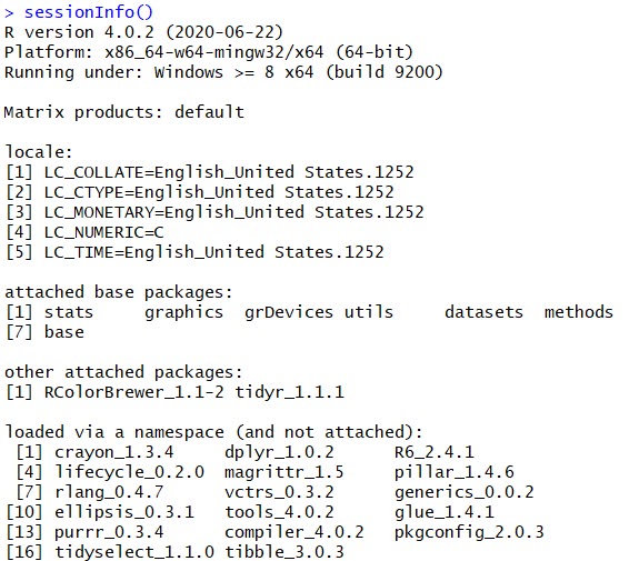 |
Example output of sessionInfo() |
Functions Introduction
makeAPlot = function(requiredValue1, requiredValue2, Value3="blue", Value4=TRUE, whereline=5, mylinecol="yellow") {
plot(requiredValue1, requiredValue2, col=Value3)abline(v=whereline, col=mylinecol)if(Value4==TRUE) {print("Hello!")}return(requiredValue1+5)}
x = 1:10
y = x^2
makeAPlot(x,y, mylinecol="red")
Output:

[1] "Hello!"
[1] 6 7 8 9 10 11 12 13 14 15
- When creating the function, indicate all your variables within function() parentheses and indicate also if they have a default value. For example, "blue" is the default for Value3.
- Any variables without a default value are required and must be defined when calling the function.
- Any variable with a default value aren't required. If you don't provide a value, the default will be used. In the example, I made my line red instead of yellow.
- Recommended: use return() at the end of the function to indicate the value you want back.
- Otherwise you get back the last object, e.g. "Hello!"
- If you create a function functionForSingleValue but want to apply it to a column, then use the Vectorize() function to create a new function
- This is useful for more complex functions where apply() can't be used
Free R courses and learning tools
- UCLA Institute for Quantitative & Computational Biosciences: Intro to R and Data Visualization - 3 day workshop videos
- Harvard: Data Science: R Basics - 8 week course (1-2 hours/week), self-paced
- University of Southern California's library R learning resources - including recorded workshops and links to textbooks
- "A Sufficient Introduction to R" by Derek L Sonderegger
R plotting resources:
- R-intro.pdf from r-project.org - vocabulary and manual
- "Things to be careful about in R" if you know other programming languages
- R code can be saved as a text file with the .R or .r extension. You don't NEED to use R Markdown as a beginner. It is optional and not particularly recommended.
- R Markdown = R code plus markdown code. It is used to create a notebook-style presentation with separate blocks of code. You may be familiar with markdown syntax if you have previously used Jyputer Lab, Jupyter Notebook, or LaTeX.
- Introduction to R Markdown (2020)
- R Markdown cheat sheet by posit (2022)
- R Markdown: new file template
- The benefit of R Markdown over regular .R scripts is that you can easily save output. I like using it when I runs statistics since I can write my code and also save the exact output.
- The downside of R Markdown is that the knitr software behind it can cause problems in certain situations (e.g. in Linux servers, or when data files are very large) so that requires additional troubleshooting.
----------------------------------------------------
Last updated: June 27, 2023


